Scattered Interpolation

In grid-based interpolation, values are define d at grid nodes, and they can be interpolated within each cell based on the values at the cell nodes.
In scattered interpolation, there are no grid cells to compute the weights of the different samples. Each sample is associated with a basic function (or weight function) of the distance to the center.

Sheppard interpolation

In this method the interpolated value is a weighted sum of the surrounding data points, normalized by the sum of the weights:
$$
s(x) = \frac{\sum_i w_i(x)s_i}{\sum_i w_i(x)}
$$
with weights set to an inverse power of the distance: $w_i(x) = (\|x-x_i\|+\epsilon)^{-p}$.
The derivative is zero at the data points, and the curve extrapolates to the average of the data values. This results in artefacts, as illustrated in the following figure:

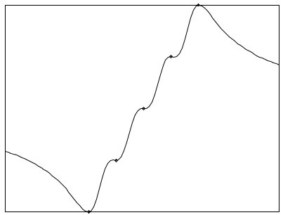
Sheppard interpolation operating on a set of colinear points. The derivative
is zero at the data points, and the curve extrapolates to the average of the data values. (source)

RBF Interpolation

Radial Basis Function (RBF) interpolation have become a popular scattered interpolation technique. I general, an RBF is a function of the form:
$$
s(x) = p(x) + \sum_i \lambda_i \phi(\|x-x_i\|)
$$
where $p(x)$ is a low-degree polynomial, and popular choices for the basic functions are:

$ \phi(r) = r^2 \log r $ for fitting smooth functions of two variables
$ \phi(r) = r$ or $\phi(r) = r^3$ for functions of three variables
$\phi(r) = e^{-cr^2}$ in neural networks
$\phi(r) = \sqrt{r^2+c^2}$ for fitting to topographical data
…

The coefficients $\lambda_i$ are computed to match the interpolation constraints: $ \sum_i \lambda_i \phi_i(x_j) = s_j$. The corresponding matrix equation to solve is:
$$
\ma{A} \ve{\lambda} = \ve{s}
$$
where $A_{ij} = \phi(\|x_i-x_j\|)$. An example is shown in the following figure.

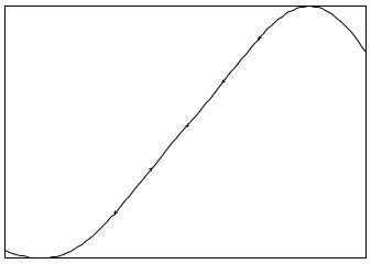
Radial basis functions φ(x) = exp(−x2 /2σ2 ), σ = 10 interpolating
the same set of colinear points as in the previous example. A different y scale is used to fit the curve.
The curve extrapolates to zero. (source)

When additional regularity conditions are set, this becomes a KKT equation system:
$$
\left( \begin{array}{cc} \ma A & \ma P^T \\ \ma P & \ma 0 \end{array} \right)
\left( \begin{array}{c} \ve \lambda \\ \ve c \end{array} \right)
=
\left( \begin{array}{c} \ve s \\ \ve 0 \end{array} \right)
$$

Francois Faure, University of Grenoble. Main page