Introduction to Finite Elements

We introduce Finite Elements for the mechanical simulation of deformable solids. In this introduction, use simplifying assumptions to more easily convey the main ideas: at initial time the object is undeformed, and the material coordinates exactly match the space coordinates. In this introduction, we focus on triangular elements in the plane.

Mesh-based model of continuous objects

Real-world material is made of atoms. We model it as a continous medium to apply differential calculus. To be simulated, a material domain is modeled using control nodes and interpolation functions, also called shape functions. In Finite Elements, the interpolations are defined within the cells of a mesh, such as the triangular mesh in the following figure.

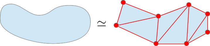
An object modeled as a mesh.

The continuity of the deformations across cell borders depends on the choice of the shape functions. The minimum required for physical plausibility is $G^0$, obtained with affine functions, as illustrated in the next figure, where sharp discontinuity is created in the middle of an initially straight line. Smoother continuity is possible using higher-degree functions.

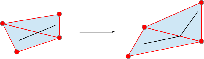
FE continuity. Linear shape functions create non-smooth deformations.

The interpolation functions are constant over time. The state (position $x$, velocity $v$) of the simulated object is represented by the values at the control nodes:
$$
\begin{eqnarray*}
\ve{x} &=& (x_0, \cdots x_{n-1})^T \\
\ve{v} &=& (v_0, \cdots v_{n-1})^T
\end{eqnarray*}
$$
We use $X$ to denote the initial values, $u(t)$ to denote the displacements over time, and $$x(t)= X + u(t)$$ to denote the current values, as illustrated in the following figure.
At each point of the domain, the simulated values (position, velocity) are entirely defined by the values at the control nodes and the interpolation functions. Let $p$ be the position of a point:
$$ p(t) = \sum_{i=0}^2 w_i x_i(t) $$
where the interpolation values $w_i$ are computed based on the positions in the initial configuration.

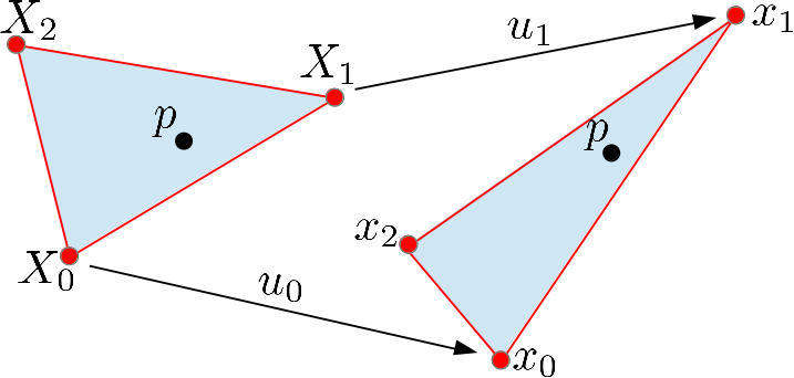
A Finite Element. Left: the reference configuration. Right: the displaced configuration.

Deformation

The local displacement of a material element can be decomposed in four different modes, illustrated in the following figure. Two of these modes are rigid: translation, rotation, while the two others are not: extension-compression corresponds to increasing or decreasing size , while shear corresponds to changing angles.

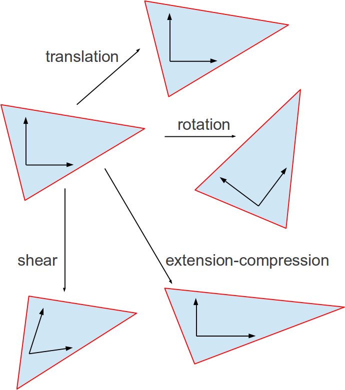
The four displacement modes of a material element.

The local displacement of the material can be represented by an initially orthonormal basis, as shown in the previous figure, called the deformation gradient and denoted $F$. It corresponds to the relation between the current and initial coordinates:
$$ F = \pd{x}{X}$$
The deformation gradient is a matrix where each column represents one of the basis vectors. It is easy to compute in triangular elements, based on the edges. Let $\bar E = (\bar E_1 \bar E_2)$ be a matrix where each column vector is an edge $\bar E_i = X_i - X_0$ of the initial triangle. This undeformed state corresponds to the identity matrix $\bar E^{-1} \bar E $. During the simulation, we compute the basis matrix $E(t)$ which columns are the current edges $E_i(t) = x_i(t)-x_0(t)$, and the new basis is computed by replacing the initial $\bar E$ with the current edge matrix:
$$ F(t) = \bar E^{-1}E(t) $$

The deformation gradient is used to compute the strain, which is a measure of the deformation. Different strains have been defined, for different purposes. One of the most popular is based on the idea that the displacement is rigid if and only if the deformation gradient is an orthogonal matrix, i.e. $F^TF = I$, where $I$ is the identity matrix. The Green-Lagrange strain tensor is therefore defined as: $$ \strain = \frac{1}{2}( F^TF-I)$$

The strain tensor is a symmetric matrix, it has thus only 3 independent entries (or 6 in 3d). The Voigt notation puts these independent values in a vector:
$$
\hat \strain = \left( \begin{array}{ccc} \strain_{xx} & \strain_{yy} & \strain_{xy} \end{array} \right)^T
$$

Energy and forces

The density of deformation energy (in $J/m^2$ in 2d, and $J/m^3$ in 3d) is a scalar value which depends on the material properties:
$$ \mathcal{w} = \frac{1}{2} \hat \strain^T H \hat \strain
$$
where matrix $H$ encodes the material properties:
$$
H = \frac{E}{1-\nu^2} \left( \begin{array}{ccc}
1 & \nu & 0 \\
\nu & 1 & 0 \\
0 & 0 & 1-\nu
\end{array} \right)
$$
where $E$ is called Young's modulus and encodes the stiffness of the material (the higher the more difficult to deform), and $\nu$ is called Poisson's ratio and encodes the material's incompressible (between 0: compressible and 1:incompressible).

The energy density is a constant across the element, thus the total deformation energy is the volume $\vol$ of the undeformed element times the energy density:
$$
\energy = \vol \energydensity
$$
and the elastic force applied to the control nodes is, as usual, derived from the energy:
$$
\ve f^T = -\pd{\energy}{\ve x} = -\pd{\energy}{\strain} \pd{\strain}{\ve x} = -\vstrain H \pd{\vstrain}{\ve x}
$$
where vector $\ve f$ concatenates the forces applied to the vertices and $\ve x$ concatenates their positions. The forces applied by the element to its nodes are split and added to the global force vector based on the node indices in the mesh, as illustrated in the following figure.

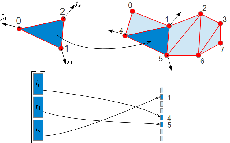
Force vector assembly. The force vector of an element (dark blue) is split and accumulated to the global force vector (light blue) based on the node indices.

The stiffness matrix is the derivative of the force with respect to the positions:
$$ \stma = \pd{\ve f}{\ve x} $$
For a triangle element in 2d, it is a $6\times 6$ symmetric matrix. For a whole mesh composed of $n$ vertices, it is a $2n \times 2n$ symmetric matrix computed by assembling all the element matrices. Each node of the element has an index in the global mesh. The element matrix is split and accumulated in the global matrix, as illustrated in the following figure.

Matrix assembly. The stiffness matrix of an element is split and accumulated to the global stiffness matrix based on the node indices.

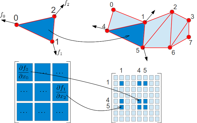
Stiffness matrix assembly. The stiffness matrix of an element (dark blue) is split and accumulated to the global stiffness matrix (light blue) based on the node indices.

Francois Faure, University of Grenoble. Main page